Sparks of Weight-Space Programming? Or Just Exploit Engineering
Cyera Research reverse engineers GPT-6 Astra’s Breakout neural network, revealing how standard logic gates and exploit engineering explain its behavior.


TL;DR: GPT-6 Astra wrote a Breakout network’s weights from scratch, and the paper saw “sparks of Weight-Space Programming, which may extend beyond what we’d expect from humans or conventional algorithms”. I’m a vulnerability researcher at Cyera Research, and I reverse engineered it by hand: it is a 15-line Python program built from standard gates, matching the network on all 4,400 possible frames and receiving identical scores. Every neuron is a threshold gate: AND, OR, NOT, or a comparator. The circuit those gates form is a lookup table that predicts the ball's landing column, minus the paddle's position, and a rule that moves the paddle toward it. The speed is impressive, but it’s a technique we know from exploit writing: start from a known source, know your primitives, read the memory layout, chain small pieces into a payload.
If you follow the technical AI space closely, you probably stumbled upon a blog post about Astra reading and writing neural network weights, which concludes:
Sean Goedecke already covered the weight reading and editing experiments (identifying the game from the weights and fixing Qwen's math) in a recent post, showing that a competent ML researcher could do the same and that it was possible to write the program as a neural network. But I set out to complete the experiment Sean skipped and I find the most interesting: writing a network from scratch.
I reverse engineered the network Astra wrote for Breakout and found it’s a short Python program built from standard gates. I’ll show you that the way Astra writes neural networks weights uses the skills of exploit engineering and nothing else.
Mapping my approach
But first, let's start by answering the following question from the blog post:
Well, as a human, I can tell you exactly what I would do step by step:
- Decide on the algorithm, implement it in Python, and evaluate it to make sure it achieves sufficient results.
- Convert it into a circuit with addition, subtraction, zero-check, and other gates (AND, OR, ...).
- Implement the circuit as a neural network.
For Go, step 1 is the hard part: you need a decent Go algorithm before there is anything to compile (and the original Go experiment also gave Astra up to 50 rounds of feedback). But nothing here is "black magic." The steps are the same for any task, and only step 1 depends on how hard the task is. That leaves one more question: how can we implement a circuit as a neural network (step 3). By now (hopefully) most engineers and computer scientists remember that any boolean circuit can be built from NAND gates alone (a universal, or functionally complete, gate).
The Go network is too big to read by hand, so I will show it on the network Astra wrote for Breakout, which is small enough to read completely. Astra's full response and weights are available in the original authors' logs.
Implementing circuits as neural networks
We first need to understand the primitives that we can use. In the case of the Breakout game experiment, we are given control of a network with three linear layers (600 → 32 → 32 → 6). The first two are each followed by a tanh activation. The last one has no activation: its six outputs are logits, one per action, and the action is sampled from their softmax.
In simple terms, each layer defines a set of variables (or neurons) of the following form:
Every neuron is a logic gate
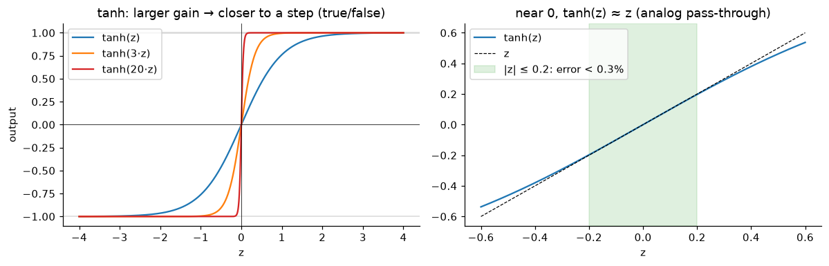
We have something better than NAND: every neuron is a threshold gate. By choosing its weights and bias, one neuron can be AND, OR, NAND, NOT, a comparator, or even a lookup table.
Implementing an AND gate
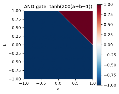
Implementing an OR gate
Implementing a NOT gate
Implementing a comparator
Reverse engineering Astra's Breakout neural network
We start by reviewing Astra's response to the user prompt:
From this response alone, we can see that there is some kind of logic embedded into the weights themselves, which strongly suggests that Astra programmed the logic into the weights similarly to what is shown above.
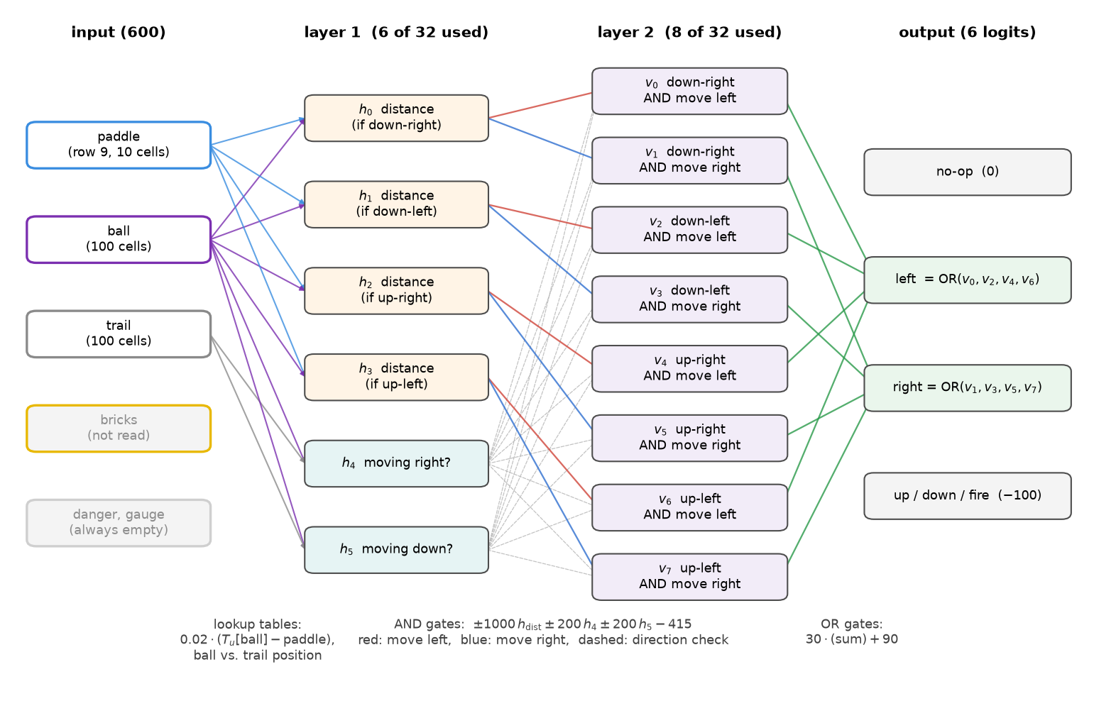
Looking at the weights, it's also clear that very few are used: only 815 of the 20,486 parameters are non-zero. Before going over the weights, here is the whole network as a circuit. We will go over it from left to right:
Game frame vectorization
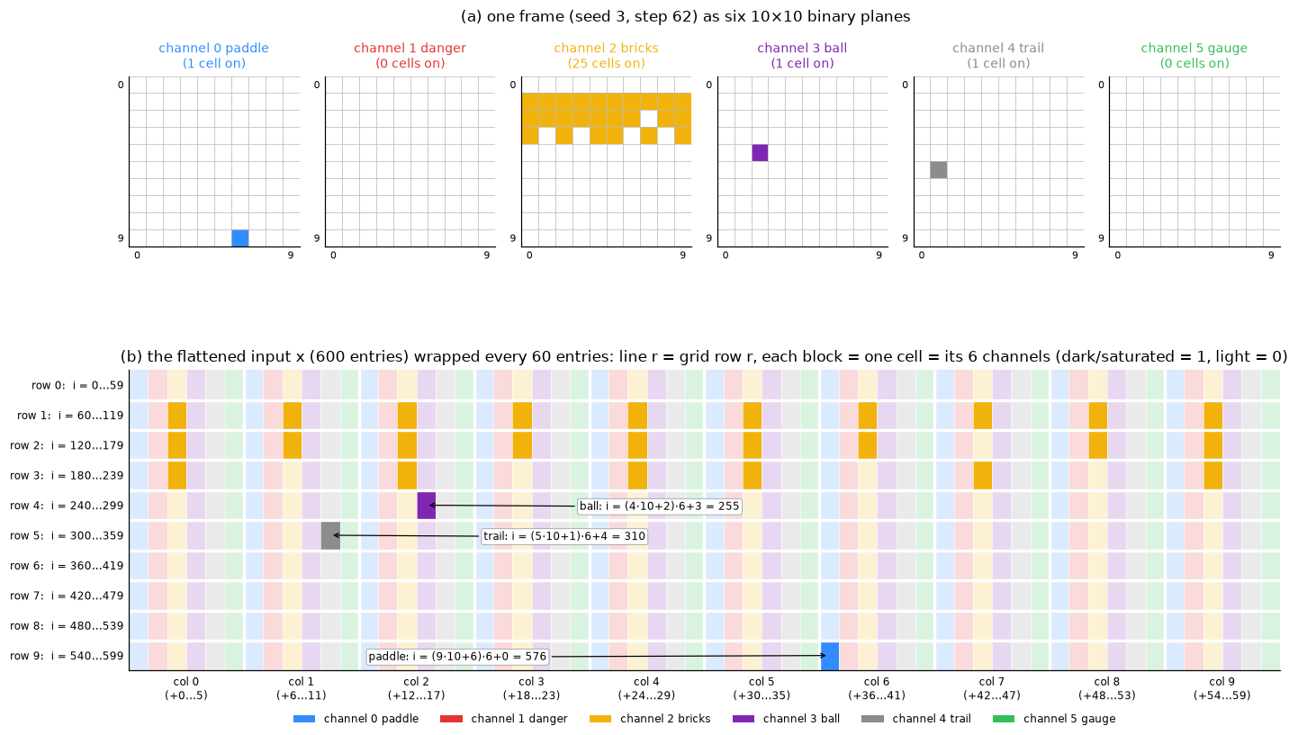
Astra writes the weights with Python slices. Since every cell takes 6 entries and every row takes 60, a stride of 6 walks along a row (in one channel) and a stride of 60 walks down a column (in one channel). For example, 540:600:6 is channel 0 in the 10 cells of row 9, and 3:600:60 is channel 3 in the 10 cells of column 0.
First layer
With the frame representation in hand, we can go through Astra's weights line by line, starting with these four:
W1[540:600:6, 0] = [0, -0.02, -0.04, -0.06, -0.08, -0.10, -0.12, -0.14, -0.16, -0.18]
W1[540:600:6, 1] = [0, -0.02, -0.04, -0.06, -0.08, -0.10, -0.12, -0.14, -0.16, -0.18]
W1[540:600:6, 2] = [0, -0.02, -0.04, -0.06, -0.08, -0.10, -0.12, -0.14, -0.16, -0.18]
W1[540:600:6, 3] = [0, -0.02, -0.04, -0.06, -0.08, -0.10, -0.12, -0.14, -0.16, -0.18]
What follows is a set of blocks, each implementing a different lookup table. For simplicity, let's focus on the first neuron's additional weights:
# Ball row 0.
W1[3:60:6, 0] = [0.16, 0.18, 0.18, 0.16, 0.14, 0.12, 0.10, 0.08, 0.06, 0.04]
# Ball row 1.
W1[63:120:6, 0] = [0.14, 0.16, 0.18, 0.18, 0.16, 0.14, 0.12, 0.10, 0.08, 0.06]
# Ball row 2.
W1[123:180:6, 0] = [0.12, 0.14, 0.16, 0.18, 0.18, 0.16, 0.14, 0.12, 0.10, 0.08]
# Ball row 3.
W1[183:240:6, 0] = [0.10, 0.12, 0.14, 0.16, 0.18, 0.18, 0.16, 0.14, 0.12, 0.10]
# Ball row 4.
W1[243:300:6, 0] = [0.08, 0.10, 0.12, 0.14, 0.16, 0.18, 0.18, 0.16, 0.14, 0.12]
# Ball row 5.
W1[303:360:6, 0] = [0.06, 0.08, 0.10, 0.12, 0.14, 0.16, 0.18, 0.18, 0.16, 0.14]
# Ball row 6: descending targets become catch-interval midpoints.
W1[363:420:6, 0] = [0.05, 0.07, 0.09, 0.11, 0.13, 0.15, 0.17, 0.18, 0.17, 0.15]
# Ball row 7.
W1[423:480:6, 0] = [0.03, 0.05, 0.07, 0.09, 0.11, 0.13, 0.15, 0.17, 0.18, 0.17]
# Ball row 8.
W1[483:540:6, 0] = [0.01, 0.03, 0.05, 0.07, 0.09, 0.11, 0.13, 0.15, 0.17, 0.18]
Those weights are multiplied by channel 3 (ball location), another lookup table that, according to Astra, assumes the ball descends down-right. Dividing this table by 0.02 to align it with the paddle location scaling, we get:
The connection to the game is easier to see when drawing ball paths on top of the table. Every cell on the path of a ball descending right shows the same column, the one where the path reaches the bottom, and the table folds exactly where the ball bounces off the right wall:
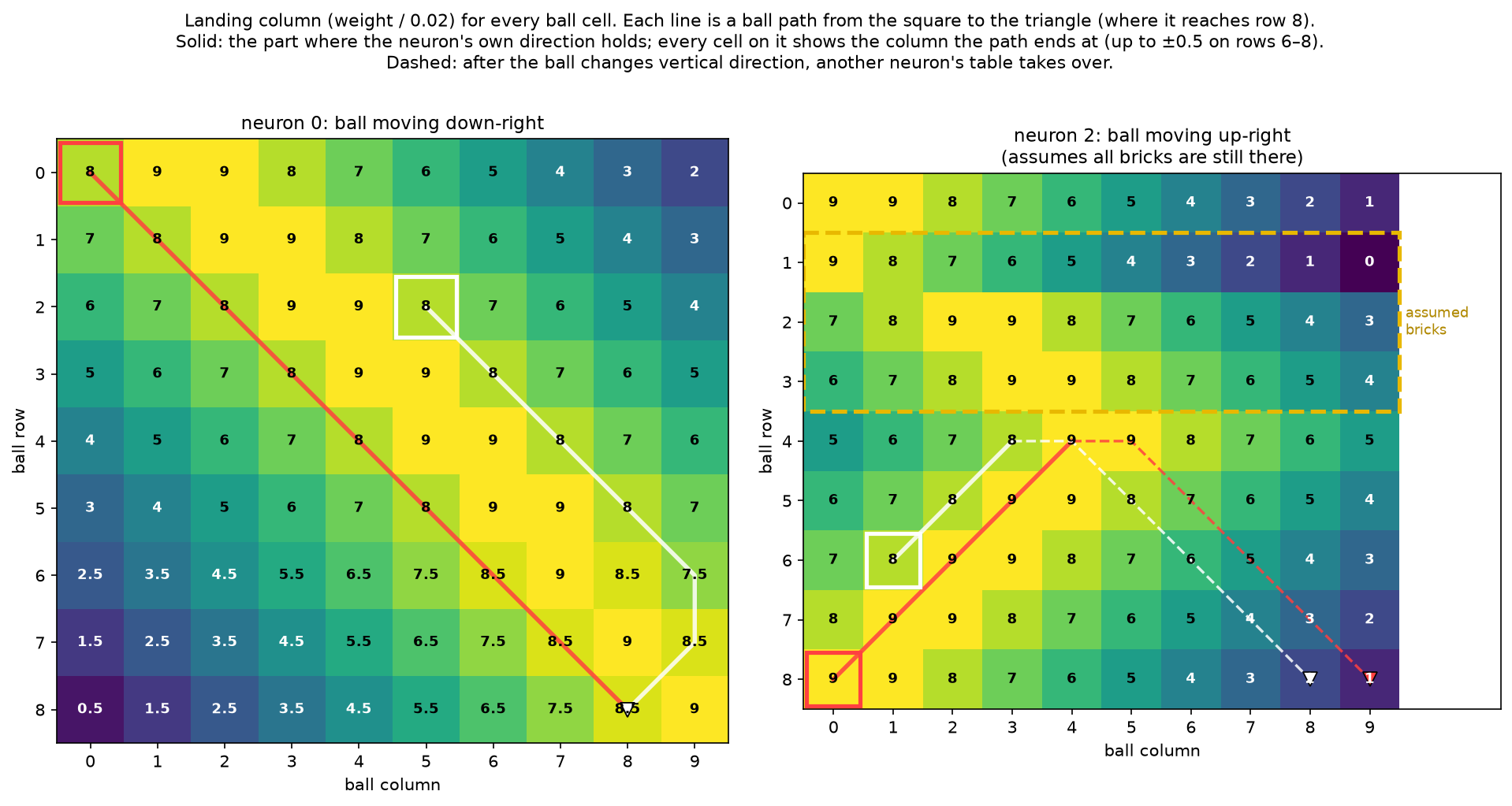
Looking at rows 0 up to 5 it is clear that they represent the column the ball arrives at when descending right, including the reflection from the right wall. Rows 6-8 contain messier values that are not entirely clear, but they will become clear in the next layer. Anyway, we now understand that the first neuron computes:
That is, the distance between the paddle and the estimated ball impact location multiplies by 0.02 to remain in the linear region. This is exactly what Astra's response says:
Neurons 1-3 are the same with their own tables. The ascending tables (neurons 2 and 3, right side of the image above) assume all the bricks are still there, since no neuron in the network reads the brick channel at all.
One more part is left for calculating those four neurons:
# Terminal-row fallback.
W1[543:600:6, 0] = [0, 0.02, 0.04, 0.06, 0.08, 0.10, 0.12, 0.14, 0.16, 0.18]
W1[543:600:6, 1] = [0, 0.02, 0.04, 0.06, 0.08, 0.10, 0.12, 0.14, 0.16, 0.18]
W1[543:600:6, 2] = [0, 0.02, 0.04, 0.06, 0.08, 0.10, 0.12, 0.14, 0.16, 0.18]
W1[543:600:6, 3] = [0, 0.02, 0.04, 0.06, 0.08, 0.10, 0.12, 0.14, 0.16, 0.18]
In practice, those weights are not used.
According to the game's Python script, this case means game over. I verified those weights are not relevant by zeroing them and running the evaluation with the same seeds on both the original and the modified weights: the metrics are identical across 1,000 episodes on each of three seeds. The same holds when zeroing every weight on a ball or trail in row 9, which means 75 of the 815 non-zero weights (9%) can never affect the game.
We have covered most of layer 1's logic. There are two more neurons to cover before we can move on to the next layer.
# Unit 4: horizontal direction, including stationary wall-reflection frames.
W1[3:600:60, 4] = 10
W1[9:600:60, 4] = 20
W1[15:600:60, 4] = 40
W1[21:600:60, 4] = 60
W1[27:600:60, 4] = 80
W1[33:600:60, 4] = 100
W1[39:600:60, 4] = 120
W1[45:600:60, 4] = 140
W1[51:600:60, 4] = 160
W1[57:600:60, 4] = 170
W1[10:600:60, 4] = -20
W1[16:600:60, 4] = -40
W1[22:600:60, 4] = -60
W1[28:600:60, 4] = -80
W1[34:600:60, 4] = -100
W1[40:600:60, 4] = -120
W1[46:600:60, 4] = -140
W1[52:600:60, 4] = -160
W1[58:600:60, 4] = -180
As the comment suggests, this neuron computes the horizontal direction of the ball taking the ball (channel 3) and the trail (channel 4) into account. The stride of 60 means each line sets a whole column, so only the columns of the ball and the trail matter, computing the following lookup table:
Finally, neuron 5's weights are similar to neuron 4's but compute whether the ball is currently ascending or descending:
# Unit 5: descending versus ascending; a stationary row-8 frame means paddle bounce.
b1[5] = 5
W1[63:120:6, 5] = 10
W1[123:180:6, 5] = 20
W1[183:240:6, 5] = 30
W1[243:300:6, 5] = 40
W1[303:360:6, 5] = 50
W1[363:420:6, 5] = 60
W1[423:480:6, 5] = 70
W1[483:540:6, 5] = 70
W1[543:600:6, 5] = 90
W1[64:120:6, 5] = -10
W1[124:180:6, 5] = -20
W1[184:240:6, 5] = -30
W1[244:300:6, 5] = -40
W1[304:360:6, 5] = -50
W1[364:420:6, 5] = -60
W1[424:480:6, 5] = -70
W1[484:540:6, 5] = -80
W1[544:600:6, 5] = -90
Second layer
Layer 2 weights are defined as follows:
# Four context-gated pairs of left/right comparisons.
W2[0, 0:2] = [-1000, 1000]
W2[1, 2:4] = [-1000, 1000]
W2[2, 4:6] = [-1000, 1000]
W2[3, 6:8] = [-1000, 1000]
W2[4, 0:8] = [200, 200, -200, -200, 200, 200, -200, -200]
W2[5, 0:8] = [200, 200, 200, 200, -200, -200, -200, -200]
b2[0:8] = -415
Third layer
Finally, the last layer is defined by the following weights:
# Near-deterministic movement when needed; otherwise no-op.
W3[0:8:2, 1] = 30
W3[1:8:2, 3] = 30
b3[:] = [0, 90, -100, 90, -100, -100]
The network
To summarize, the whole network can be written back as the following program:
To verify, I compared astra_program with the network on every frame the game can produce: every ball cell, every possible trail cell, and every paddle column (4,400 frames). They agree on 100% of them, and astra_program gets the same score as the network. Going the other way, from this program back to the weights, is exactly the gate construction from the beginning of this post.
Is the program at least clever? Not really. Astra implements a short program that predicts where the ball will land and moves the paddle there. It ignores the brick channel, assumes every brick is still in place while the ball is ascending, corrects its guess frame by frame, and never aims for the bricks. It only has to keep the ball alive, which is what the score mostly rewards.
This way of writing weights from scratch is not surprising
Hopefully by now you are convinced that writing neural networks without training is feasible even for a human. That said, you might prefer to write a compiler to make your life easier.
I would like to conclude by showing you the similarities between writing Astra's weights and writing an exploit.
Given these similarities, the results are not surprising for Astra: OpenAI reports that it solves 42.4% of the ExploitGym benchmark in its own testing, with no time limit (OpenAI) Writing weights from scratch with no tools, on the first try, in about eight minutes, is still an impressive piece of engineering. But it is the skill of an exploit engineer (Astra is a very good one), not a sign of something beyond what we'd expect from humans or conventional algorithms.